Understanding Statistical Power
2020-11-22
Part 2 of 3 on a series of notes covering margin of error, power, and sample size calculations.
Notes, with questions and examples, taken from the following reading: https://sphweb.bumc.bu.edu/otlt/MPH-Modules/BS/BS704_Power/BS704_Power_print.html
Type I and Type II Errors, and their relationship to Power
In hypothesis testing there are two kinds of errors that can be made when deciding whether to reject the null hypothesis or not:
Type I Error
A type I error is falsely rejecting $h_0$ (the null hypothesis) when it is actually true, i.e. a false positive. Imagine a doctor looking at a man and telling him he's pregnant. The level of significance in a hypothesis test, $\alpha$ (alpha), is the probability of a type I error occuring:
$\alpha$ = P(Type I Error) = P(Rejct $H_0$ | $H_0$ is True)
We can use alpha as a control for the probability of making a type I error.
Type II Error
A type II error is not rejecting $h_0$ when it it's actually false, i.e. a false negative. This time, the doctor looks at a pregnant lady and tells her she's got to start exercising to get rid of that giant bump in her belly. The probability of making a type II error is denoted as $\beta$ (beta):
$\beta$ = P(Type II Error) = P(Do not reject $H_0$ | $H_0$ is False)
Statistical Power
The power of a hypothesis test is the probability that $H_0$ will be correctly rejected when it is false. In other words, its the probability of detecting an effect if it actually exists. This is the probability of not making a type II error:
Power = 1 - $\beta$ = 1 - P(Do not reject $H_0$ | $H_0$ is False)
A good hypothesis tests has a low significance threshold (small $\alpha$) and high power (small $\beta$). Power is a single piece in a puzzle of four interconnected parts:
- The chosen significance level of the hyptothesis test, $\alpha$
- The desired power of the test, (1 - $\beta$)
- The sample size, which determines the variability of the parameter of interest
- The effect size, the difference observed in the parameter of interest that denotes a meaningful difference (determined through domain knowledge)
Power analysis involves estimating one of these variables given we know the values of the other three.
Example
Say we have some parameter of interest in a population that we want to make an inference on. We want to test the following hypothesis about this parameter:
The Null Hypothesis $H_0$: the population mean $\mu$ for the parameter is 90. $\mu$ = 90
The Alternative Hypothesis $H_A$: the population mean $\mu$ for the parameter is not 90. $\mu$ $\neq$ 90
Here are the conditions for the test: - We want to test a hypothesis with a significance level of $\alpha$ = 0.05, i.e. the probability of a false positive is only 5%. - The test is two sided, meaning we are testing to see if the parameter of interest is lower or higher than our null hypothesis - From previous tests on the population we can safely estimate that the standard deviation $\sigma$ of the parameter is 20. $\sigma$ = 20 - To conduct this test we select a sample of n = 100
To conduct the test we compute the parameter's sample mean $\bar{X}$ and then decide whether it provides enough evidence to support the alternative hypothesis. To do this we compute a test statistic and compare it to the appropriate critical value; since we know the variability of the parameter we can use a Z test.
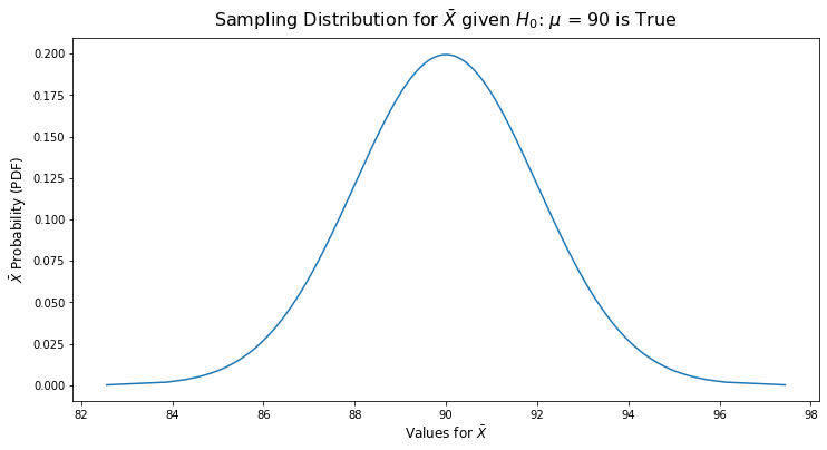
If the null hypothesis is true ($\mu$ = 90) then we are likely to select a sample whose mean is close to 90. However it's possible to have a sample mean that is much larger or smaller than 90.
We can use the Central Limit Theorum here: when n is sufficiently large (in this case n=100 is enough), the distribution of sample means is approximately normal with a mean of:
$$ \mu_X = \mu $$
The standard error of our sample can be calculated as:
$$ SE = \frac{\sigma}{\sqrt{n}} = \frac{20}{\sqrt{100}} = 2.0 $$
If the null hypothesis is true, then it is possible to observe any sample mean from the sampling distribution below:
import numpy as np
from scipy.stats import norm
import matplotlib.pyplot as plt
h0_true_mean = 90
standard_deviation = 20
sample_size = 100
standard_error = standard_deviation / np.sqrt(sample_size)

h0_sample_dist = norm(h0_true_mean, standard_error)

x_range = h0_sample_dist.ppf(np.linspace(0.0001, 0.9999, num=1000))

plt.figure(figsize=(12,6))
plt.plot(x_range, h0_sample_dist.pdf(x_range))

plt.title("Sampling Distribution for $\\bar{X}$ given $H_0$: $\mu$ = 90 is True",
          fontsize=16, pad=10)
plt.xlabel("Values for $\\bar{X}$", fontsize=12)
plt.ylabel("$\\bar{X}$ Probability (PDF)", fontsize=12)

plt.show()
Given this sampling distribution, we determine critical lower and upper values at which we reject $H_0$ based on our chosen significance ($\alpha = 0.05$) and the decision that this will be a two-sided test:
upper_rejection_cutoff = h0_sample_dist.ppf(0.975) # 2.5% probability of occuring at or after this threshold
lower_rejection_cutoff = h0_sample_dist.ppf(0.025) # 2.5% probability of occuring at or before this threshold

print(f"Upper rejection cutoff: {upper_rejection_cutoff}")
print(f"Lower rejection cutoff: {lower_rejection_cutoff}")
Upper rejection cutoff: 93.9199279690801
Lower rejection cutoff: 86.0800720309199
Speaking in terms of the Z test, we would take the calculated sample mean $\bar{X}$ and convert it into a Z score. We'd then find this Z score's probability on a standard normal distribution and if it was less than 5% (i.e. outside of our lower and upper rejection cutoffs), we would reject $H_0$.
In this example the critical values for a two-sided test with $\alpha$ = 0.05 are 86.06 and 93.92 (-1.96 and 1.96 on the Z scale), so the decision rule becomes reject $H_0$ if $\bar{X}$ $\leq$ 86.06 or if $\bar{X}$ $\geq$ 93.92.
plt.figure(figsize=(12,6))
plt.plot(x_range, h0_sample_dist.pdf(x_range))

plt.axvline(lower_rejection_cutoff, color='r', linestyle='--',
            label=f'{lower_rejection_cutoff}')
plt.axvline(upper_rejection_cutoff, color='r', linestyle='--',
            label=f'{upper_rejection_cutoff}')


lower_rejection_range = np.linspace(h0_sample_dist.ppf(0.0001),
                                    lower_rejection_cutoff,
                                    num=1000)

upper_rejection_range = np.linspace(upper_rejection_cutoff,
                                    h0_sample_dist.ppf(0.9999),
                                    num=1000)

non_rejection_range = np.linspace(lower_rejection_cutoff,
                                  upper_rejection_cutoff,
                                  num=1000)

plt.fill_between(non_rejection_range,
                 0,
                 h0_sample_dist.pdf(non_rejection_range),
                 color='green',
                 alpha=0.5)

plt.fill_between(lower_rejection_range,
                 0,
                 h0_sample_dist.pdf(lower_rejection_range),
                 color='red',
                 alpha=0.5)

plt.fill_between(upper_rejection_range,
                 0,
                 h0_sample_dist.pdf(upper_rejection_range),
                 color='red',
                 alpha=0.5)


plt.title("Rejection Region for Test $H_0$: $\\mu$ = 90 vs. $H_A$: $\\neq$ 90 at $\\alpha$ = 0.05",
          fontsize=16, pad=10)
plt.xlabel("Values for $\\bar{X}$", fontsize=12)
plt.ylabel("$\\bar{X}$ Probability (PDF)", fontsize=12)
plt.legend()

plt.show()
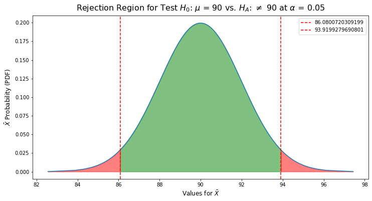
The red areas that aren't between the two rejection lines represent the probability of a Type I error, which are the values for sample mean $\bar{X}$ whose probabilities sum to $\alpha$ = 0.05. If $\bar{X}$ is in these regions, we reject $H_0$ with a 5% probability of making a type I error. The green area represents the chosen range where $\bar{X}$ supports the null hypothesis, so we do not reject $h_0$.
If we suppose the alternative hypothesis, $H_A$ is true ($\mu$ $\neq$ 90) and that the true mean is actually 94, this is what the distributions of the sample mean look like for the null and alternate hypotheses:
true_mean = 94

x_range = np.linspace(80,100, num=1000)

hA_sample_dist = norm(true_mean, standard_error)

plt.figure(figsize=(12,6))

plt.axvline(true_mean, linestyle='--', label='$\mu$ = 94')
plt.axvline(lower_rejection_cutoff, color='r', linestyle='--',
            label=f'{lower_rejection_cutoff}')
plt.axvline(upper_rejection_cutoff, color='r', linestyle='--',
            label=f'{upper_rejection_cutoff}')

plt.plot(x_range, h0_sample_dist.pdf(x_range), color='b', label='$H_0$')
plt.plot(x_range, hA_sample_dist.pdf(x_range), color='r', label='$H_A$')

false_neg_range = np.linspace(lower_rejection_cutoff,
                              upper_rejection_cutoff, num=1000)
plt.fill_between(false_neg_range,
                 0,
                 hA_sample_dist.pdf(false_neg_range),
                 color='red',
                 alpha=0.5)

power_range = np.linspace(upper_rejection_cutoff,
                          100, num=1000)
plt.fill_between(power_range,
                 0,
                 hA_sample_dist.pdf(power_range),
                 color='green',
                 alpha=0.5)

plt.title("Distribution of $\\bar{X}$ under $H_0$: $\\mu$ = 90 and under $H_A$: $\\mu$ = 94 ")
plt.xlabel("Values for $\\bar{X}$", fontsize=12)
plt.ylabel("$\\bar{X}$ Probability (PDF)", fontsize=12)
plt.legend()

plt.show()
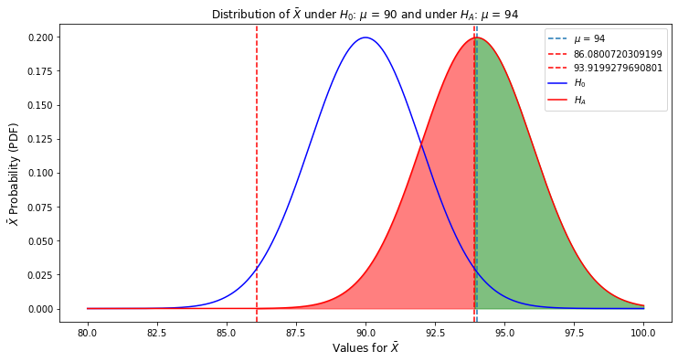
If the true mean is 94, then the alternative hypothesis $H_A$ is true. The probability of a type II error, $\beta$, is the red shaded area: this is the overlap between the alternate hypothesis' distribution has with the "do not reject region" of the null hypothesis.
The test's power, i.e. the probability of a true positive, rejecting $h_0$ when it is truly false, is the green shaded area to the right of the null hypothesis' upper rejection cutoff (as set by $\alpha$). It can be calculated as the probability of $\bar{X}$ being a value greater than $H_0$'s upper rejection cutoff of 93.91, given $H_A$ is true (1 - probability of beta).
To do this we can put the upper rejection cutoff $\bar{X}$ = 93.91 in terms of its associated Z statistic:
$$ Power = 1 - \beta = P(\bar{X} > 93.91 | H_A) $$
$$ Power = P\left(Z > \frac{93.92 - 94}{\frac{20}{\sqrt{100}}}\right) $$
$$ Power = P\left(Z > -0.04\right) $$
We can convert the Z score of -0.04 using the cumulative density function, which will represent the probablility of drawing values less than or equal to -0.04 on a standard normal distribution
beta_calc = (upper_rejection_cutoff - true_mean)/standard_error
norm.cdf(beta_calc)
0.4840322065576678
This gives us a beta $\beta$ of 0.484 (the probability of $\bar{X}$ being less or equal to 93.91, giving us a false negative). From there we can just subtract this value from 1 to get the probability of that not happening (true positive):
$$ Power = 1 - \beta = P(\bar{X} > 93.91 | H_A) = 1 - 0.484 = 0.516 $$
Therefore, the given power of this test between $H_0$ and $H_A$ is 51.6% (not great). $\beta$ can also be calculated from our $H_A$ distribution object, by obtaining the CDF at $H_0$'s upper rejection region:
beta_from_dist = hA_sample_dist.cdf(upper_rejection_cutoff)
power = round(1 - beta_from_dist, 4) * 100
print(f"The power of this hypothesis test is {power}%")
The power of this hypothesis test is 51.6%
$\beta$ and power are related to $\alpha$, the variance of the outcome and the effect size (i.e. the difference in the parameter of interest between $H_0$ and $H_A$). If we increased $\alpha$ from 0.05 to 0.10, the upper rejection limit of $H_0$ would shift to the left and be larger, increasing the test's power. While this would give the test higher power, it would also reduce the confidence we could have in the test.
The effect size and variance of the outcome affect power in clear ways: - Increase the desired effect size between $H_0$ and $H_A$ to move their respective distributions further away from each other, reducing their overlap - Gathering more samples and reducing the variance of $H_0$ and $H_A$'s distributions will also reduce their overlap
Using the exact same components as the plot above, here is what the test's power becomes when $H_0$: $\mu$ = 90 and $H_A$: $\mu$ = 98, an effect size of 8 units:
hA_mean = 98

x_range = np.linspace(80,110, num=1000)

hA_sample_dist = norm(hA_mean, standard_error)

plt.figure(figsize=(12,6))

plt.axvline(lower_rejection_cutoff, color='r', linestyle='--',
            label=f'{lower_rejection_cutoff}')
plt.axvline(upper_rejection_cutoff, color='r', linestyle='--',
            label=f'{upper_rejection_cutoff}')

plt.plot(x_range, h0_sample_dist.pdf(x_range), color='b', label='$H_0$')
plt.plot(x_range, hA_sample_dist.pdf(x_range), color='r', label='$H_A$')

false_neg_range = np.linspace(lower_rejection_cutoff,
                              upper_rejection_cutoff, num=1000)
plt.fill_between(false_neg_range,
                 0,
                 hA_sample_dist.pdf(false_neg_range),
                 color='blue',
                 alpha=0.5)

power_range = np.linspace(upper_rejection_cutoff,
                          110, num=1000)
plt.fill_between(power_range,
                 0,
                 hA_sample_dist.pdf(power_range),
                 color='green',
                 alpha=0.5)

plt.title("Distribution of $\\bar{X}$ under $H_0$: $\\mu$ = 90 and under $H_A$: $\\mu$ = 94 ")
plt.xlabel("Values for $\\bar{X}$", fontsize=12)
plt.ylabel("$\\bar{X}$ Probability (PDF)", fontsize=12)
plt.legend()
<matplotlib.legend.Legend at 0x7ff6971a7390>
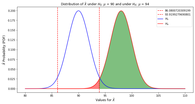
Calculating the Power for this test by obtaining $\beta$ from $H_A$'s distribution variable:
beta_from_dist = hA_sample_dist.cdf(upper_rejection_cutoff)
power = round(1 - beta_from_dist, 4) * 100
print(f"The power of this hypothesis test is {power}%")
The power of this hypothesis test is 97.92999999999999%