Stats Review: The Most Dangerous Equation
2021-06-05
Notes from Causal Inference for the Brave and True
https://matheusfacure.github.io/python-causality-handbook/03-Stats-Review-The-Most-Dangerous-Equation.html
Stats Review: The Most Dangerous Equation
The Standard Error of Mean is a dangerous equation to not know:
$SE = \frac{\sigma}{\sqrt{n}}$
With $\sigma$ as the standard deviation and $n$ as the sample size.
Looking at a dataset of ENEM scores (Brazillian standardized high school scores similar to SAT) from different schools over three years:
import warnings
warnings.filterwarnings('ignore')

import pandas as pd
import numpy as np
from scipy import stats
import seaborn as sns
from matplotlib import pyplot as plt
from matplotlib import style
style.use("fivethirtyeight")
df = pd.read_csv("data/enem_scores.csv")
df.sort_values(by="avg_score", ascending=False).head(10)
| year | school_id | number_of_students | avg_score | |
|---|---|---|---|---|
| 16670 | 2007 | 33062633 | 68 | 82.97 |
| 16796 | 2007 | 33065403 | 172 | 82.04 |
| 16668 | 2005 | 33062633 | 59 | 81.89 |
| 16794 | 2005 | 33065403 | 177 | 81.66 |
| 10043 | 2007 | 29342880 | 43 | 80.32 |
| 18121 | 2007 | 33152314 | 14 | 79.82 |
| 16781 | 2007 | 33065250 | 80 | 79.67 |
| 3026 | 2007 | 22025740 | 144 | 79.52 |
| 14636 | 2007 | 31311723 | 222 | 79.41 |
| 17318 | 2007 | 33087679 | 210 | 79.38 |
Initial observation is that top performing schools seem to have a low number of students - Taking a look at the top 1%:
plot_data = (df
             .assign(top_school = df["avg_score"] >= np.quantile(df["avg_score"], .99))
             [["top_school", "number_of_students"]]
             .query(f"number_of_students<{np.quantile(df['number_of_students'], .98)}"))

plt.figure(figsize=(6,6))
sns.boxplot(x="top_school", y="number_of_students", data=plot_data)
plt.title("Number of Students in 1% top schools (right)")
Text(0.5, 1.0, 'Number of Students in 1% top schools (right)')
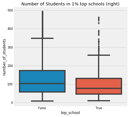
The data does suggest that top schools do have less students, which makes sense intuitively.
The trap appears when we just take this at face value and make decisions on it: - What if we looked at bottom 1% of schools too?
q_99 = np.quantile(df['avg_score'], .99)
q_01 = np.quantile(df['avg_score'], .01)
plot_data = (df
             .sample(10000)
             .assign(group = lambda d: np.select([d['avg_score'] > q_99,
                                                  d['avg_score'] < q_01],
                                                 ['Top', 'Bottom'],
                                                 'Middle')))
plt.figure(figsize=(10,5))
sns.scatterplot(y="avg_score",
                x="number_of_students",
                hue="group",
                data=plot_data)
plt.title("ENEM Score by Number of Students in the School")
Text(0.5, 1.0, 'ENEM Score by Number of Students in the School')
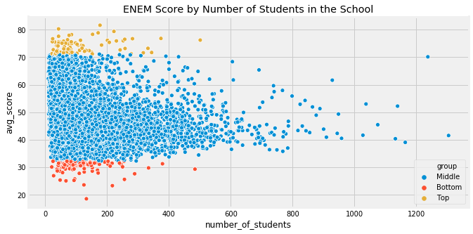
plot_data.groupby('group')['number_of_students'].median()
group
Bottom     95.5
Middle    104.0
Top        77.0
Name: number_of_students, dtype: float64
- Bottom 1% of schools also have less students as well
As the number of units in a sample grows, the variance of the sample decreases and averages get more precise. - Smaller samples can have a lot of variance in their expected outcome variables due to chance
Speaks to a fundamental fact about the reality of information: it is always imprecise. - The question becomes: can we quantify how imprecise it is? - Probabilty is an acceptance of the lack of certainty in our knowledge and the development of methods for dealing with our ignorance
The Standard Error of our Estimates
We can test and see if the $ATE$ from the last chapter (GPA scores for students in traditional classrooms vs. online) was significant. First step is calculating the standard error $SE$:
data = pd.read_csv("data/online_classroom.csv")
online = data.query("format_ol ==  1")["falsexam"]
face_to_face = data.query("format_ol == 0 & format_blended == 0")["falsexam"]
def se(y: pd.Series):
    return y.std() / np.sqrt(len(y))
print(f"SE for Online: {se(online)}")
print(f"SE for Face to Face: {se(face_to_face)}")
SE for Online: 1.5371593973041635
SE for Face to Face: 0.8723511456319106
Confidence Intervals
The Standard Error $SE$ of an estimate is a measure of confidence.
Has a different interpretation depending on the different views of statistics (Frequentist and Bayesian).
Frequentist view: - The data is a manifestation of a true data generating process - If we could run multiple experiments and collect multiple datasets, all would resemble the underlying process
For the sake of an example lets say that the true distribution of a student's test score is normal distribution $N(\mu, \sigma^{2})$ with $\mu = 74$ and $\sigma = 2$.
Run 10,000 experiments, collecting 500 units per sample:
true_std = 2
true_mean = 74

n = 500
def run_experiment():
    return np.random.normal(true_mean, true_std, 500)

np.random.seed(42)

plt.figure(figsize=(8,5))
freq, bins, img = plt.hist([run_experiment().mean() for _ in range(10000)],
                           bins=40,
                           label="Experiment's Mean")
plt.vlines(true_mean, ymin=0, ymax=freq.max(), linestyles="dashed", label="True Mean")
plt.legend()
<matplotlib.legend.Legend at 0x7fbb7ab33e90>
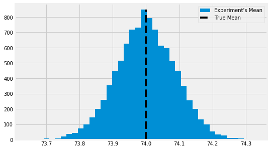
- This is the distribution of sample means; the sample distribution
- The standard error is the standard deviation of this distribution
- With the standard error we can create an interval that will contain the true mean 95% of the time (95% CI)
- We take the desired $Z$ score for the normal distribution, in this case Z = 1.96 for 95% CDF and $\pm$ that multipled by $SE$ to get the confidence interval around a point estimate
- $SE$ serves as our estimate for the means' distribution of our experiments
from scipy.stats import norm
z = norm.ppf(0.975)
z
1.959963984540054
np.random.seed(321)
exp_data = run_experiment()
exp_se = exp_data.std() / np.sqrt(len(exp_data))
exp_mu = exp_data.mean()
ci = (exp_mu - z * exp_se, exp_mu + z * exp_se)
print(ci) # 95% of the time the data's true mean will fall within this interval
(73.83064660084463, 74.16994997421483)
We can construct a confidence interval for $ATE$ on GPA scores in our classroom example:
def ci(y: pd.Series, confidence = 0.975):
    return (y.mean() - norm.ppf(confidence) * se(y), y.mean() + norm.ppf(confidence) * se(y))
print(f"95% CI for Online: {ci(online)}")
print(f"95% CI for Face to Face: {ci(face_to_face)}")
95% CI for Online: (70.62248602789292, 76.64804014231983)
95% CI for Face to Face: (76.8377077560225, 80.2572614106441)
- We can see that there's no overlap between the two groups' CIs: this is evidence that the results were not by chance
- Very likely that there is a significant causal decrease in academic performance once you switch from face to face to online classes.
There is a nuance to confidence intervals: - The population mean is constant; you shouldn't really say that the confidence interval contains the population mean with 95% chance. Since it is constant, it is either in the interval or not. - The 95% refers to the frequency that such confidence intervals, computed in many other studies, contain the true mean. - 95% confidence in the algorithm used to compute the 95% CI, not on a particular interval itself - Bayesian statistics and the use of probability intervals are able to say that an interval contains the distribution mean 95% of the time.
Hypothesis Testing
Is the difference in two means significant, or statistically different from zero/another value? - Recall that the sum or difference of normal distributions is also a normal distribution - The resulting mean will be the sum or difference of the two distributions' means, while the variance will always be the sum of variance
$$N(\mu_1, \sigma_{1}^{2}) - N(\mu_2, \sigma_{2}^{2}) = N(\mu_1 - \mu_2, \sigma_{1}^{2} + \sigma_{2}^{2})$$ $$N(\mu_1, \sigma_{1}^{2}) + N(\mu_2, \sigma_{2}^{2}) = N(\mu_1 + \mu_2, \sigma_{1}^{2} + \sigma_{2}^{2})$$
np.random.seed(123)

n1 = np.random.normal(4, 3, 30000)
n2 = np.random.normal(1, 4, 30000)
n_diff = n1 - n2

sns.distplot(n1, hist=False, label="N(4,3)")
sns.distplot(n2, hist=False, label="N(1,4)")
sns.distplot(n_diff, hist=False, label="N(4,3) - N(1,4) = N(3,5)")
<matplotlib.axes._subplots.AxesSubplot at 0x7fbb7ec4a550>
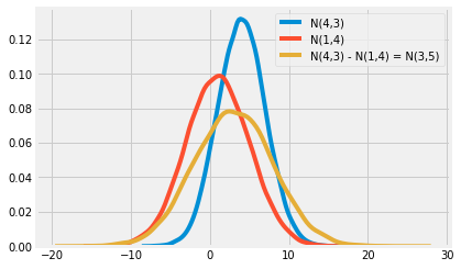
- If we take the distribution of the means of our two groups and subtract one from the other, we get a third distribution equaling the difference in the means and the standard deviation of the distribution will be the square root of the sum of the standard deviations:
$$ \mu_{diff} = \mu_1 - \mu_2 $$ $$ SE_{diff} = \sqrt{SE_1 + SE_2} = \sqrt{\frac{\sigma_{1}^{2}}{n_1} + \frac{\sigma_{2}^{2}}{n_2}} $$
Constructing the distribution of the difference with the classroom example:
diff_mu = online.mean() - face_to_face.mean()
diff_se = np.sqrt(online.var()/len(online) + face_to_face.var()/len(face_to_face))
ci = (diff_mu - 1.96 * diff_se, diff_mu + 1.96 * diff_se)
ci
(-8.376410208363357, -1.4480327880904964)
Plot the confidence interval with the distribution of differences between online and face-to-face groups:
diff_dist = stats.norm(diff_mu, diff_se)
x = np.linspace(diff_mu - 4 * diff_se, diff_mu + 4 * diff_se, 100)
y = diff_dist.pdf(x)

plt.plot(x,y)
plt.vlines(ci[0], ymin=0, ymax = diff_dist.pdf(ci[0]))
plt.vlines(ci[1], ymin=0, ymax = diff_dist.pdf(ci[1]), label = "95% CI")
plt.legend()
plt.show()
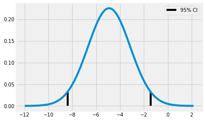
- We can say that we're 95% that the true difference between groups falls within this interval of (-8.37, -1.44)
We can create a z statistic by dividing the difference in means by the standard error of the differences:
$$ z = \frac{\mu_{diff} - H_0}{SE_{diff}} = \frac{(u_1 - u_2) - H_0}{\sqrt{\frac{\sigma_{1}^{2}}{n_1} + \frac{\sigma_{2}^{2}}{n_2}}} $$
- Where $H_0$ is the value which we want to test our difference against
- The z statistic is a measure of how extreme the observed difference is
- With the null hypothesis we ask: "how likely is it that we would observe this difference if the true/population difference was actually zero/[insert whatever your null hypothesis is]?"
- The z statistic is computed through the data to be standardized to the standard normal distribution; i.e. if the difference were indeed zero we would see z be within two standard deviations of the mean 95% of the time.
z = diff_mu / diff_se
print(z)
-2.7792810791031064
x = np.linspace(-4, 4, 100)
y = stats.norm.pdf(x, 0, 1)


plt.plot(x, y, label="Standard Normal")
plt.vlines(z, ymin=0, ymax= .05, label="Z statistic", color="C1")
plt.legend()
plt.show()
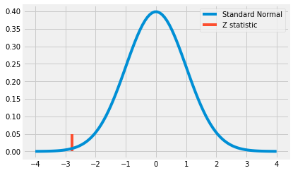
- We can see that the Z statistic is a pretty extreme value (more than 2 standard devations away from the mean)
- Interesting point about hypothesis tests: they're less conservative than checking if the 95% CIs from the two groups overlap; i.e. they can overlap but still be a result that's statistically significant
- If we pretend that the face-to-face group has an average score of 74 with a standard error of 7 and the online group has an average score of 71 with a standard error of 1:
ctrl_mu, ctrl_se = (71, 1)
test_mu, test_se = (74, 7)

diff_mu = test_mu - ctrl_mu
diff_se = np.sqrt(ctrl_se + test_se)

groups = zip(['Control', 'Test', 'Diff'], [[ctrl_mu, ctrl_se],
                                           [test_mu, test_se],
                                           [diff_mu, diff_se]])

for name, stats in groups:
    print(f"{name} 95% CI:", (stats[0] - 1.96 * stats[1], stats[0] + 1.96 * stats[1],))
Control 95% CI: (69.04, 72.96)
Test 95% CI: (60.28, 87.72)
Diff 95% CI: (-2.5437171645025325, 8.543717164502532)
- The CI for the difference between groups contains 0, so maybe the example provided by the author above isn't a great one... moving on...
P-Values
- From Wikipedia: “the p-value is the probability of obtaining test results at least as extreme as the results actually observed during the test, assuming that the null hypothesis is correct”
- i.e. the probablity of seeing the results given that the null hypothesis is true
- It is not equal to the probability of the null hypothesis being true!
-
Not $P(H_{0} \vert data)$, but rather $P(data \vert H_{0})$
-
To obtain, just compute the area under the standard normal distribution before or after the z statistic
- Simply plug the z statistic into the CDF of the standard normal distribution:
print(f'P-value: {norm.cdf(z)}')
P-value: 0.0027239680835564706
- Means that there's a 0.2% chance of observing this z statistic given the null hypothesis is true; this falls within the accepted significance level to reject the null hypothesis
- The p-value avoids us having to specify a confidence level
- We can know exactly at which confidence our test will pass or fail though, given the p-value; with a P-value of 0.0027, we will have significance up to the 0.2% level
- A 95% CI and a 99% CI for the difference won't contain zero, but a 99.9% CI will:
diff_mu = online.mean() - face_to_face.mean()
diff_se = np.sqrt(online.var()/len(online) + face_to_face.var()/len(face_to_face))
print("95% CI:", (diff_mu - norm.ppf(.975)*diff_se, diff_mu + norm.ppf(.975)*diff_se))
print("99% CI:", (diff_mu - norm.ppf(.995)*diff_se, diff_mu + norm.ppf(.995)*diff_se))
print("99.9% CI:", (diff_mu - norm.ppf(.9995)*diff_se, diff_mu + norm.ppf(.9995)*diff_se))
95% CI: (-8.37634655308288, -1.4480964433709733)
99% CI: (-9.464853535264012, -0.3595894611898425)
99.9% CI: (-10.72804065824553, 0.9035976617916743)
Key Ideas
- The standard error enables us to put degrees of certainty around our estimates by enabling us to calculate confidence intervals around our point estimates as well as the statistical significance of a result given hypothesis testing
- Wrapping everything up, we can create an A/B testing function to automate all the work done above:
def AB_test(test: pd.Series, control: pd.Series, confidence=0.95, h0=0):
    mu1, mu2 = test.mean(), control.mean()
    se1, se2 = test.std()/np.sqrt(len(test)), control.std()/np.sqrt(len(control))

    diff = mu1 - mu2
    se_diff = np.sqrt(test.var()/len(test) + control.var()/len(control))

    z_stats = (diff - h0)/se_diff
    p_value = norm.cdf(z_stats)

    def critical(se): return -se*norm.ppf((1 - confidence)/2)

    print(f"Test {confidence*100}% CI: {mu1} +- {critical(se1)}")
    print(f"Control {confidence*100}% CI: {mu2} +- {critical(se2)}")
    print(f"Test - Control {confidence*100}% CI: {diff} +- {critical(se_diff)}")
    print(f"Z statistic: {z_stats}")
    print(f"P-Value: {p_value}")
AB_test(online, face_to_face)
Test 95.0% CI: 73.63526308510637 +- 3.0127770572134565
Control 95.0% CI: 78.5474845833333 +- 1.7097768273108005
Test - Control 95.0% CI: -4.912221498226927 +- 3.4641250548559537
Z statistic: -2.7792810791031064
P-Value: 0.0027239680835564706