Introduction to Causality
2021-03-15
Notes from Causal Inference for the Brave and True
https://matheusfacure.github.io/python-causality-handbook/01-Introduction-To-Causality.html
Introduction to Causality
Data Science is kind of like a cup of beer, with a little bit of foam on the top: - The beer is statistical foundations, scientific curiousity, passion for difficult problems - The foam is the hype and unrealistic expectations that will disappear eventually
Focus on what makes your work valuable.
Answering a Different Kind of Question
- ML doesn't bring intelligence, it brings predictions
- Must frame problems as prediction ones, and it's not so good at explaining causation
Causal questions are everywhere: - Does X cause an increase in sales? - Does higher education lead to higher earnings? - Does immigration cause unemployment to go up?
ML and correlation-type predictions don't work for these questions.
We always hear that correlation isn't causation: - Explaining why takes some understanding - This book explains how to figure out when correlation is causation
When Association is Causation
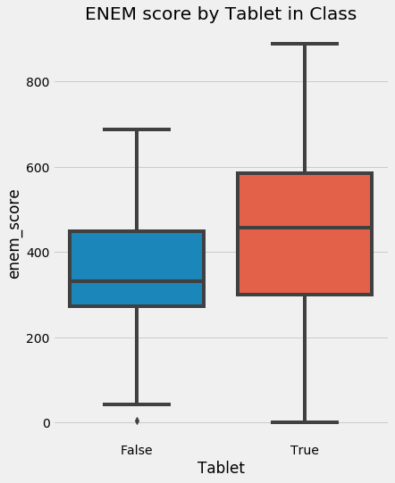
We can intuitively understand why correlation doesn't necessarily mean causation: - If someone says that schools that give their students tablets to work with perform better, we can quickly point out that these schools are probably better funded, richer families, etc. - We can't say that tablets make students perform better, but they're associated/correlated with better performance (due to underlying factors)
import pandas as pd
import numpy as np
from scipy.special import expit
import seaborn as sns
import matplotlib.pyplot as plt
from matplotlib import style
style.use("fivethirtyeight")

np.random.seed(123)
n = 100
tuition = np.random.normal(1000, 300, n).round()
tablet = np.random.binomial(1, expit((tuition - tuition.mean()) / tuition.std())).astype(bool)
enem_score = np.random.normal(200 - 50 * tablet + 0.7 * tuition, 200)
enem_score = (enem_score - enem_score.min()) / enem_score.max()
enem_score *= 1000

df = pd.DataFrame(dict(enem_score=enem_score, Tuition=tuition, Tablet=tablet))
df
| enem_score | Tuition | Tablet | |
|---|---|---|---|
| 0 | 227.622953 | 674.0 | False |
| 1 | 219.079925 | 1299.0 | True |
| 2 | 400.889622 | 1085.0 | False |
| 3 | 122.761509 | 548.0 | False |
| 4 | 315.064276 | 826.0 | False |
| ... | ... | ... | ... |
| 95 | 451.019929 | 1309.0 | True |
| 96 | 113.288467 | 675.0 | True |
| 97 | 116.042782 | 591.0 | False |
| 98 | 266.238616 | 1114.0 | True |
| 99 | 297.431514 | 886.0 | True |
100 rows × 3 columns
plt.figure(figsize=(6,8))
sns.boxplot(y="enem_score", x="Tablet", data=df).set_title("ENEM score by Tablet in Class")
plt.show()
$T_i$ is the treatment intake for unit $i$: - 1 if unit $i$ received the treatment - 0 otherwise
$Y_i$ is the observed outcome variable of interest for unit $i$
The fundamental problem of causal inference is we can never observe the same unit with/without treatment: - Like two diverging roads in life... you always wonder what could have been </3 - Potential outcomes are talked about a lot, denoting what would/could have happened if some treatment was taken - Sometimes call the outcome that happened "factual", and the one that didn't as "counterfactual"
$Y_{0i}$ is the potential outcome for unit $i$ without the treatment
$Y_{1i}$ is the potential outcome for the same unit $i$ with the treatment
In our example: - $Y_{1i}$ is the academic performance of student $i$ if they are in a classroom with tablets - $Y_{0i}$ otherwise - If the student gets the tablet, we can observe $Y_{1i}$, if not we can observe $Y_{0i}$ - Each counterfactual is still defined, we just can't see it - a potential outcome
With potential outcomes we can define the treatment effect:
$ Y_{1i} - Y_{0i} $
- Of course we can never know the treatment effect directly because we can only observe one of the potential outcomes
Focus on easier things to estimate/measure:
Average treatment effect:
$ ATE = E[Y_1 - Y_{0}] $
- Where $E[...]$ is the expected value
Average treatment effect on the treated:
$ ATET = E[Y_1 - Y_{0} \vert T = 1] $
Pretending we could see both potential outcomes (a gift from the causal inference gods): - Collected data on 4 schools - We know if they gave tablets to students and their score on a test - $T = 1$ is treatment (getting the tablets) - $Y$ is test score
data = pd.DataFrame(dict(i = [1,2,3,4],
                         y0 = [500,600,700,800],
                         y1 = [450,600,600,750],
                         t = [0,0,1,1],
                         y = [500,600,600,750],
                         te = [-50,0,-200,50],)) # TE is treatment effect
data
| i | y0 | y1 | t | y | te | |
|---|---|---|---|---|---|---|
| 0 | 1 | 500 | 450 | 0 | 500 | -50 |
| 1 | 2 | 600 | 600 | 0 | 600 | 0 |
| 2 | 3 | 700 | 600 | 1 | 600 | -200 |
| 3 | 4 | 800 | 750 | 1 | 750 | 50 |
$ATE$ would be the mean of $TE$:
data.te.mean()
-50.0
- Tablets reduced the academic performance of students, on average, by 50 pts
$ATET$:
data[data.t == 1].te.mean()
-75.0
- For schools that were treated, tablets reduced academic performance by 75 pts on average
In reality (where we can't observe counterfactuals) the data would look like:
reality_data = pd.DataFrame(dict(i = [1,2,3,4],
                                 y0 = [500,600,np.nan,np.nan],
                                 y1 = [np.nan,np.nan,600,750],
                                 t = [0,0,1,1],
                                 y = [500,600,600,750],
                                 te = [np.nan,np.nan,np.nan,np.nan],))
reality_data
| i | y0 | y1 | t | y | te | |
|---|---|---|---|---|---|---|
| 0 | 1 | 500.0 | NaN | 0 | 500 | NaN |
| 1 | 2 | 600.0 | NaN | 0 | 600 | NaN |
| 2 | 3 | NaN | 600.0 | 1 | 600 | NaN |
| 3 | 4 | NaN | 750.0 | 1 | 750 | NaN |
You can't just take the mean of the treated and compare it with the mean of the untreated to try and answer the question of causality: - That's committing a grave sin: mistaking association for causation
Bias
The main enemy of causal inference.
Schools with tablets are likely richer than those without; i.e. the treated schools (with tablets) are not the same as untreated schools (without tablets, likely poorer). The $Y_0$ of the treated is different from the $Y_0$ of the untreated.
Leverage your understanding of how the world works: - The $Y_0$ of the treated schools is likely larger than untreated schools for other reasons - Schools that can afford tablets can also afford other factors that contribute to better the scores
Association is measured by $E[Y \vert T = 1] - E[Y \vert T = 0]$ - e.g. the average test score for schools with tablets minus the average test score of those without them
Causation is measured by $E[Y_{1} - Y_{0}]$
To see how they relate:
First, take the association measurement and replace observed outcomes with potential outcomes
$E[Y \vert T = 1] - E[Y \vert T = 0] = E[Y_{1} \vert T = 1] - E[Y_{0} \vert T = 0]$
Now lets add and subtract $E[Y_{0} \vert T = 1]$, the counterfactual outcome. What would have been the outcome of the treated group, had they not received treatment.
$E[Y \vert T = 1] - E[Y \vert T = 0] = E[Y_{1} \vert T = 1] - E[Y_{0} \vert T = 0] + E[Y_{0} \vert T = 1] - E[Y_{0} \vert T = 1]$
Through reordering the terms and merging some expectations we get:
$E[Y \vert T = 1] - E[Y \vert T = 0] = E[Y_{1} - Y_{0} \vert T = 1] + E[Y_{0} \vert T = 1] - E[Y_{0} \vert T = 0]$
Where - $E[Y_{1} - Y_{0} \vert T = 1]$ is $ATET$ - $E[Y_{0} \vert T = 1] - E[Y_{0} \vert T = 0]$ is our $BIAS$ term
Association is equal to the treatment effect on the treated plus a bias term: - The bias is given by how the treated and control group differ before the treatment; in the case neither of them has received the treatment - In this example, we think that $E[Y_0 \vert T = 0] < E[Y_0 \vert T = 1]$; that schools who can afford to give tablets are better than those that can't, regardless of the tablets treatment
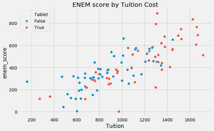
Bias arises from many things we can't control changing together with the experiment (confounding variables). - e.g. treated and untreated schools don't just differ on tablets, but on tuition cost, location, teachers, etc. - To claim that tablets improve performance, we would need schools with and without them to be, on average, similar to each other
plt.figure(figsize=(10,6))
sns.scatterplot(x="Tuition", y="enem_score", hue="Tablet", data=df, s=70).set_title("ENEM score by Tuition Cost")
Text(0.5, 1.0, 'ENEM score by Tuition Cost')
We know the problem, and here's the solution:
If $E[Y_{0} \vert T = 0] = E[Y_{0} \vert T = 1]$, then association is causation! - This is saying that the treatment and control group are comparable before the treatment - If we could observe $Y_{0}$ for the treated group, then its outcome would be the same as the untreated
This makes the bias term vanish in association, leaving only $ATET$:
$E[Y \vert T = 1] - E[Y \vert T = 0] = E[Y_{1} - Y_{0} \vert T = 1] + 0$
If $E[Y_{0} \vert T = 0] = E[Y_{0} \vert T = 1]$, the causal impact on the treated is the same as in the untreated (because they are similar).
$E[Y_{1} - Y_{0} \vert T = 1] = E[Y_{1} \vert T = 1] - E[Y_{0} \vert T = 1]$
$\hspace{3.35cm} = E[Y_{1} \vert T = 1] - E[Y_{0} \vert T = 0]$
$\hspace{3.35cm} = E[Y \vert T = 1] - E[Y \vert T = 0]$
Hence the difference in means becomes the causal effect:
$E[Y \vert T = 1] - E[Y \vert T = 0] = ATE = ATET$
Causal inference is all about finding clever ways to remove bias through experimentation, making the treatment and control groups comparable so that all the difference we can see between them is only the average treatment effect.
Key Ideas
Association is not causation, but it can be (if there are no other differences between the groups being tested, AKA bias).
Potential outcome notation and the idea of counterfactuals - two potential realities, but only one of them can be measured (the funadamental problem of causal inference).
"What happens in a man's life is already written. A man must move through life as his destiny wills."
"Yes, but each man is free to live as he chooses. Though they seem opposite, both are true".